Relative density ratio for 1D Gaussians

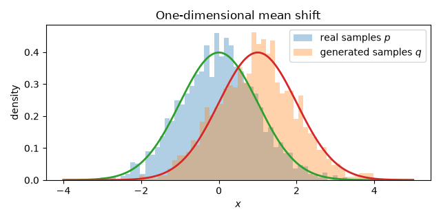
This notebook-style example follows the one-dimensional mean-shift experiment from the original RDR repository. We compare

\[p=\mathcal N(0,1), \qquad q=\mathcal N(1,1)\]

and estimate

\[r(x)=\frac{2p(x)}{p(x)+q(x)}.\]

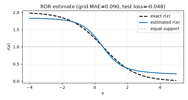
The Gaussian densities are known, so the learned curve can be compared with the exact RDR. Values above one favor the real distribution p and values below one favor the generated distribution q.

Author: RDR contributors %% Imports and reproducibility —————————

import numpy as np
import matplotlib.pyplot as plt
import torch

from rdr import Divergence, RDRTrainer

SEED = 123
np.random.seed(SEED)
torch.manual_seed(SEED)

<torch._C.Generator object at 0x7f6b0ffd88f0>

Generate real and generated samples

n_real, n_generated = 2_000, 1_600
generated_mean = 1.0
x_real = torch.randn(n_real, 1)
x_generated = torch.randn(n_generated, 1) + generated_mean

grid = torch.linspace(-4.0, 5.0, 500).reshape(-1, 1)


def normal_pdf(x, mean=0.0, std=1.0):
    return torch.exp(-0.5 * ((x - mean) / std) ** 2) / (
        std * torch.sqrt(torch.tensor(2.0 * torch.pi))
    )


p_grid = normal_pdf(grid, mean=0.0)
q_grid = normal_pdf(grid, mean=generated_mean)
true_rdr = 2.0 * p_grid / (p_grid + q_grid)

fig, ax = plt.subplots(figsize=(6.4, 3.2))
ax.hist(x_real.numpy(), bins=60, density=True, alpha=0.35, label="real samples $p$")
ax.hist(x_generated.numpy(), bins=60, density=True, alpha=0.35, label="generated samples $q$")
ax.plot(grid, p_grid, linewidth=2)
ax.plot(grid, q_grid, linewidth=2)
ax.set(title="One-dimensional mean shift", xlabel="$x$", ylabel="density")
ax.legend()
fig.tight_layout()

Define the ratio network

The final line contains the only output sigmoid. The trainer consumes and returns this already-bounded ratio without applying another activation.

class RatioNet1D(torch.nn.Module):
    def __init__(self):
        super().__init__()
        self.body = torch.nn.Sequential(
            torch.nn.Linear(1, 32),
            torch.nn.Tanh(),
            torch.nn.Linear(32, 32),
            torch.nn.Tanh(),
            torch.nn.Linear(32, 1),
        )

    def forward(self, x):
        return 2.0 * torch.sigmoid(self.body(x))

Fit the RDR estimator

trainer = RDRTrainer(
    RatioNet1D(),
    divergence=Divergence.HELLINGER,
    lr=1e-3,
    weight_decay=0.0,
    device="cpu",
)
_, losses = trainer.fit(
    x_real,
    x_generated,
    num_epochs=500,
    batch_size=256,
    validation_fraction=0.2,
    test_fraction=0.1,
    split_seed=SEED,
    early_stopping_patience=25,
    early_stopping_start=50,
    min_delta=1e-5,
    restore_best=True,
    verbose=False,
)

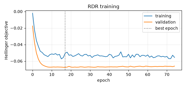
fig, ax = plt.subplots(figsize=(6.4, 3.0))
ax.plot(losses, label="training")
ax.plot(trainer.validation_history, label="validation")
if trainer.best_epoch is not None:
    ax.axvline(trainer.best_epoch, color="0.4", linestyle=":", label="best epoch")
ax.set(title="RDR training", xlabel="epoch", ylabel="Hellinger objective")
ax.legend()
ax.grid(alpha=0.25)
fig.tight_layout()

Compare the exact and estimated ratios

estimated_rdr = trainer.score(grid).cpu().reshape(-1, 1)
mae = torch.mean(torch.abs(estimated_rdr - true_rdr)).item()

fig, ax = plt.subplots(figsize=(6.4, 3.4))
ax.plot(grid, true_rdr, "k--", linewidth=2.2, label="exact $r(x)$")
ax.plot(grid, estimated_rdr, linewidth=2.2, label="estimated $r(x)$")
ax.axhline(1.0, color="0.5", linestyle=":", label="equal support")
ax.set(
    xlabel="$x$",
    ylabel="$r(x)$",
    ylim=(-0.05, 2.05),
    title=f"RDR estimate (grid MAE={mae:.3f}, test loss={trainer.test_loss:.3f})",
)
ax.legend()
ax.grid(alpha=0.2)
fig.tight_layout()
plt.show()