Relative density ratio for 2D Gaussian mixtures

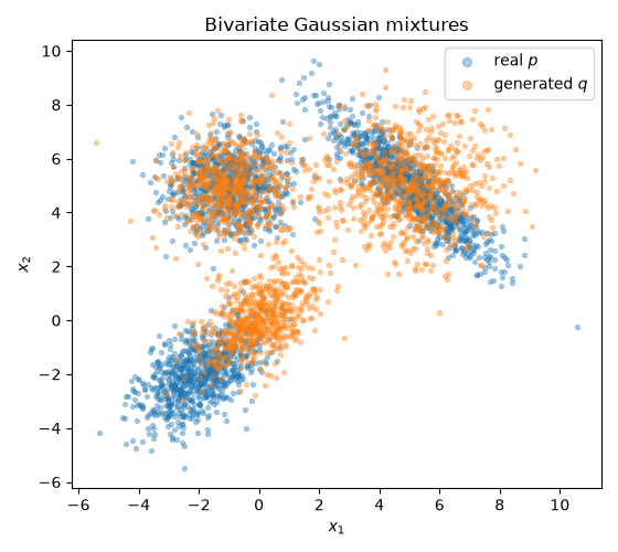
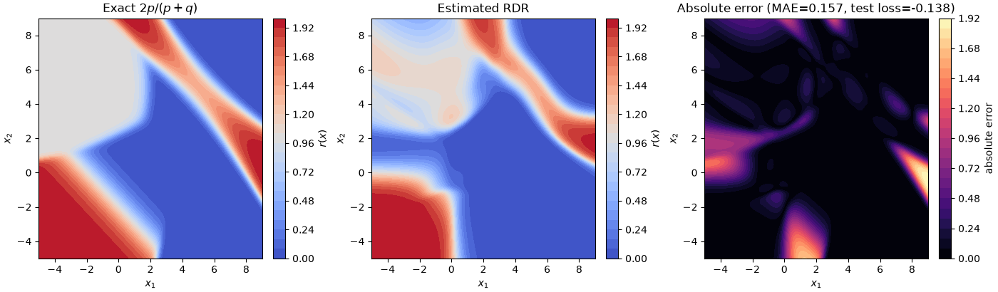
This example adapts the bivariate Gaussian-mixture experiment from the original RDR repository. The distributions share two mixture components, but their lower-left component is shifted. The learned RDR should therefore be near one in shared regions and depart from one where their probability masses differ.

Author: RDR contributors %% Imports and helpers ——————-

import numpy as np
import matplotlib.pyplot as plt
from matplotlib.colors import TwoSlopeNorm
import torch

from rdr import Divergence, RDRTrainer

SEED = 123
rng = np.random.default_rng(SEED)
torch.manual_seed(SEED)


def sample_gaussian_mixture(n, weights, means, covariances, generator):
    labels = generator.choice(len(weights), size=n, p=weights)
    samples = np.empty((n, 2), dtype=np.float32)
    for component in range(len(weights)):
        selected = labels == component
        samples[selected] = generator.multivariate_normal(
            means[component], covariances[component], selected.sum()
        )
    return samples


def gaussian_mixture_density(points, weights, means, covariances):
    density = np.zeros(len(points), dtype=np.float64)
    for weight, mean, covariance in zip(weights, means, covariances):
        difference = points - mean
        inverse = np.linalg.inv(covariance)
        exponent = np.einsum("ni,ij,nj->n", difference, inverse, difference)
        normalizer = 2.0 * np.pi * np.sqrt(np.linalg.det(covariance))
        density += weight * np.exp(-0.5 * exponent) / normalizer
    return density

Generate the two mixtures

These parameters mirror the structure of experiments/Sim_20D.py in the upstream repository while keeping this example focused on its 2D base case.

weights = np.array([0.3, 0.3, 0.4])
means_p = np.array([[-2.0, -2.0], [-1.0, 5.0], [5.0, 5.0]])
means_q = np.array([[0.0, 0.0], [-1.0, 5.0], [5.0, 5.0]])
covariances_p = np.array(
    [[[1.0, 0.5], [0.5, 1.0]], [[1.0, 0.0], [0.0, 1.0]], [[2.0, -1.8], [-1.8, 2.0]]]
)
covariances_q = np.array(
    [[[1.0, 0.5], [0.5, 1.0]], [[1.0, 0.0], [0.0, 1.0]], [[2.0, 0.0], [0.0, 2.0]]]
)

x_real_np = sample_gaussian_mixture(2_500, weights, means_p, covariances_p, rng)
x_generated_np = sample_gaussian_mixture(2_000, weights, means_q, covariances_q, rng)
x_real = torch.from_numpy(x_real_np)
x_generated = torch.from_numpy(x_generated_np)

fig, ax = plt.subplots(figsize=(5.6, 5.0))
ax.scatter(*x_real_np.T, s=8, alpha=0.35, label="real $p$")
ax.scatter(*x_generated_np.T, s=8, alpha=0.35, label="generated $q$")
ax.set(title="Bivariate Gaussian mixtures", xlabel="$x_1$", ylabel="$x_2$")
ax.legend(markerscale=2)
fig.tight_layout()

Define and train the ratio network

class RatioNet2D(torch.nn.Module):
    def __init__(self):
        super().__init__()
        self.body = torch.nn.Sequential(
            torch.nn.Linear(2, 64),
            torch.nn.Tanh(),
            torch.nn.Linear(64, 64),
            torch.nn.Tanh(),
            torch.nn.Linear(64, 1),
        )

    def forward(self, x):
        # Exactly one bounded output activation.
        return 2.0 * torch.sigmoid(self.body(x))


trainer = RDRTrainer(
    RatioNet2D(),
    divergence=Divergence.HELLINGER,
    lr=1e-3,
    weight_decay=0.0,
    device="cpu",
)
_, losses = trainer.fit(
    x_real,
    x_generated,
    num_epochs=700,
    batch_size=256,
    validation_fraction=0.2,
    test_fraction=0.1,
    split_seed=SEED,
    early_stopping_patience=30,
    early_stopping_start=75,
    min_delta=1e-5,
    restore_best=True,
    verbose=False,
)

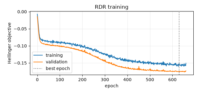
fig, ax = plt.subplots(figsize=(6.4, 3.0))
ax.plot(losses, label="training")
ax.plot(trainer.validation_history, label="validation")
if trainer.best_epoch is not None:
    ax.axvline(trainer.best_epoch, color="0.4", linestyle=":", label="best epoch")
ax.set(title="RDR training", xlabel="epoch", ylabel="Hellinger objective")
ax.legend()
ax.grid(alpha=0.25)
fig.tight_layout()

Evaluate on a regular grid

x_axis = np.linspace(-5.0, 9.0, 170)
y_axis = np.linspace(-5.0, 9.0, 170)
xx, yy = np.meshgrid(x_axis, y_axis)
grid_np = np.column_stack([xx.ravel(), yy.ravel()]).astype(np.float32)

p_grid = gaussian_mixture_density(grid_np, weights, means_p, covariances_p)
q_grid = gaussian_mixture_density(grid_np, weights, means_q, covariances_q)
true_rdr = (2.0 * p_grid / (p_grid + q_grid + 1e-15)).reshape(xx.shape)
estimated_rdr = trainer.score(torch.from_numpy(grid_np)).cpu().numpy().reshape(xx.shape)
grid_mae = np.mean(np.abs(estimated_rdr - true_rdr))

Compare exact RDR, estimated RDR, and error

fig, axes = plt.subplots(1, 3, figsize=(14.0, 4.1), constrained_layout=True)
norm = TwoSlopeNorm(vmin=0.0, vcenter=1.0, vmax=2.0)

for ax, values, title in zip(
    axes[:2], [true_rdr, estimated_rdr], ["Exact $2p/(p+q)$", "Estimated RDR"]
):
    image = ax.contourf(xx, yy, values, levels=30, cmap="coolwarm", norm=norm)
    ax.set(title=title, xlabel="$x_1$", ylabel="$x_2$")
    fig.colorbar(image, ax=ax, label="$r(x)$")

error = axes[2].contourf(xx, yy, np.abs(estimated_rdr - true_rdr), levels=30, cmap="magma")
axes[2].set(
    title=f"Absolute error (MAE={grid_mae:.3f}, test loss={trainer.test_loss:.3f})",
    xlabel="$x_1$",
    ylabel="$x_2$",
)
fig.colorbar(error, ax=axes[2], label="absolute error")
plt.show()